We made it a whole year!
Our son just turned 1 year old!! We made it through the first year, with all its trials, twists and turns. We’re all happier, older, more full of love, and I hope a little bit wiser.
To celebrate, I’m going to prove how much of a nerdy PhDad I am. I’m going to spend my saturday night fitting growth models to his height and weight observations we took at the various doctors’ appointments last year, instead of working on my thesis or a talk I’m giving next week.
Really, I’m interested in 2 things: (1) trying to fit the data with a model, and (2) trying to predict my son’s adult height. I’m envisioning this as a series of blog posts that I update with new data points. Ideally, I would be able to update my model fit as time goes on, and if this website persists long enough, I would be able to (in)validate my model with the true observations in about 18-22 years. Hah!
Data
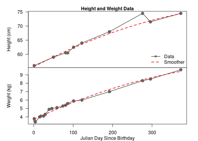
First, we need the data. I used a handy phone app to record heights and weights whenever they were observed at the various appointments. These data have been collected into the table at the bottom of this post. This shows the observations of height and weight (if the were taken) on julian day \(j\) since his birthday (\(j = 1\)).
We can visualise the data on a multi-panel plot, and fit a smoother to each quantity to take a look at the average behaviour. I’ve done this below. Notice that we have a lot more weight observations than height observations in the first four months. All I can say about that is breastfeeding is HARD, and my wife is a rockstar. The other thing you might notice is that this data follows a fairly steady trend. The deviations in the height plots are likely observation errors (height data for infants is noisy). On the other hand, the deviations for weight observations are likely process variation, as doctors’ offices have fairly accurate scales that take an average weight over a time period; this variation can be explained by changes in my son’s diet and the occasional growth spurt.
Modeling human growth
There are several papers on modeling human growth in the medical literature that I just turned up in a quick google scholar search. Most are based on the Infancy-Childhood-Puberty (ICP) model (Karlberg 1987), which seems to have been the standard for most of the last 30 years. Recently, an updated approach was derived based on phenomenological universalities (Gliozzi et al. 2012), but to my untrained eye this model overlaps a lot with the ICP model.
I’m going to use a different model, though. You might have guessed it, given that I’m a fisheries student, but I’m going to use a von Bertalanffy model, which I will refer to as the vonB model for short. This is because neither of the above models from the medical literature satisfy both of my requirements for this post. They’ll certainly fit to my son’s data (who knows how well - maybe another post) but they won’t predict adult height from infant observations given that they switch model structures for different life stages, so I’m going to pass on them.
Defining the model
I’m going to use the form of the vonB model that de-correlates the asymptotic (adult) length \(L_{\infty}\) from the growth ‘rate’1 \(K\) (Schnute 1981; Francis 2016): \[ L_a = L_1 + (L_2 - L_1) \cdot \frac{e^{-K A_1} - e^{-K a}}{e^{-K A_1} - e^{-K A_2}}. \] Here, \(L_a\) is the length at age \(a\), in years, \(K\) is the rate of change in length per unit time, and \(L_1\) and \(L_2\) are the lengths at ages \(A_1\) and \(A_2\), ages that are chosen to be representative of early and late stage lengths, respectively.
I’m going to have to modify this model a little bit to use the data I have. First, humans stand up, so I’m modeling height \(H\), not growth \(L\) - a completely aesthetic changes of variables. Second, I have observations with time-steps in days, not years, so I’m going to have to use a different rate \(K' = K/365\), making the formula \[ H_d = H_1 + (H_2 - H_1) \cdot \frac{e^{-K' D_1} - e^{-K' d}}{e^{-K' D_1} - e^{-K' D_2}}, \] where \(D_1\) and \(D_2\) are ages in days for \(H_1\) and \(H_2\), respectively.
I should be able to estimate this model from the data, but I foresee at least one challenge. This is a three parameter model (\(L_1\), \(L_2\), and \(K\)). I technically have enough data to estimate three parameters, but I don’t have any data that represents the late stage height \(H_2\) (we’ve got some time to wait for that). I’m going to attempt extrapolating out to 18 years, by setting \(D_2 = 365\) to see what it does, and encouraging the model to 20 years by setting a prior distribution on the \(K\) parameter, with a mean value intended to produce something close to a heuristic prediction of adult height. My wife is 158 cm, and I am 178cm, so our son’s predicted maximum height according to this Mayo Clinic method is \[ \mu_{H_\infty} = \frac{158 + 178 + 13}{2} = 174.5 \mbox{cm}. \]
Implementing the vonB model R
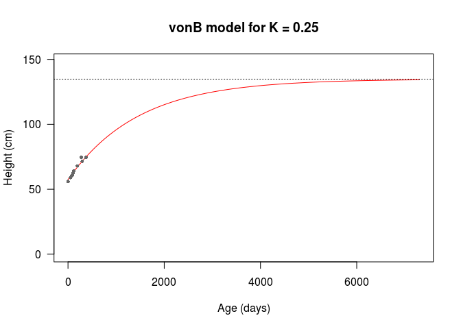
So, let’s get into the knitty-gritty. We’re going to optimise later, so I’m going to define a vonB() function, which takes the number of days \(d\) and the model parameters defined above as arguemnts. I’m going to set function default argument values based on the observations, with \(D_1 = 100\), \(D_2 = 365\), and assume a yearly \(K = 0.25\) for now.
# First, create a function to calculate the
# height at a given day d. Leading parameters
# H_1, H_2 and K are separated from D values
# as pars are estimated model parameters passed
# in from the log-likelihood function
vonB <- function( d = 1,
                  pars = c( H_1 = 62.5,
                            H_2 = 74.5,
                            K = 0.25 ),
                  D = c(100,365) )
{
  # Recover pars
  H_1 <- pars[1]
  H_2 <- pars[2]
  K   <- pars[3]/365

  # Recover D values
  D_1 <- D[1]
  D_2 <- D[2]

  # Run calculation
  H_d <- H_1 + (H_2 - H_1) * (exp(-K*D_1) - exp(-K*d)) /( exp(-K*D_1) - exp(-K*D_2) )

  # Return H_d
  return(H_d)
}
Fitting by eye
If I run the model with the default values, we can see that it fits the data we have pretty well by eye. The only caveat is that the asymptotic height is 134.79cm, which is low based on my heuristic estimate of 174.5cm above. This is likely because my randomly chosen initial \(K\) value is too high, leading the growth to saturate at a lower asymptotic height.
Thanks to my functional workflow, it’s easy to change values and produce more growth curves.
H2 <- vonB( d = 1:14600, pars = c( H_1 = 62.5,
H_2 = 74.5,
K = 0.16 ) )
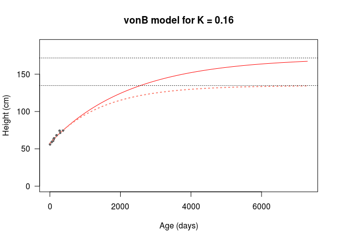
Hinf2 <- max(H2)After some fiddling around, I can get a better asymptotic height from \(K = 0.16\), which produces an asymptotic height of 171.73cm. I’ve plotted this new curve and the previous model on the axes below.
Optimisation
Let’s optimise! First, we need a negative log-posterior density function, which we’re going to use in an optim() call. We’ll run the optimisation with the default values, which is a short interval between \(D_1 = 100\) and \(D_2 = 365\). I’m going to add three prior distributions to penalise deviations from (1) the last observed height of 74.5cm at 1 year old, (2) the \(K = 0.16\) growth rate that I eye-balled to give an adult height similar to the heuristic from the Mayo Clinic, and (3) an improper Jeffreys prior on the observation error \(\sigma\).
Assuming the residuals between the model and the data are normally distributed, we have the likelihood function \[ \mathcal{L} = \prod_{i} \frac{1}{2\sqrt{\pi\sigma^2}} e^{-\frac{(H_d - \hat{H}_d)^2}{2\sigma^2}}. \] This is implemented in the following code chunk, along with the priors on \(H_2\), \(K\), and \(\sigma\).
# Define negative log posterior function,
# we're going to model the H1, H2 and K
# values on the log scale, and we need to
# model
vonB_negLogPost <- function(  theta = c( logH_1 = log(62.5),
                                         logH_2 = log(74.5),
                                         logK = log(0.16),
                                         logsigma = 0 ),
                              data = growthData,
                              D = c(100,365),
                              H2Prior = c(74.5, 74.5),
                              KPrior = c(.16, .16/2) )
{
  # Exponentiate leading pars of vonB
  pars <- c(  H_1 = exp(theta[1]),
              H_2 = exp(theta[2]),
              K   = exp(theta[3]) )

  # uncertainty in the observations
  sigma <- exp(theta["logsigma"])

  # Calculate expected observations in a new column
  # of the data frame, then residuals,
  # and then the negative-log-likelihood (with
  # normalising scalar omitted)
  data <- data %>%
          mutate( expHeight = vonB(j, pars = pars, D = D),
                  resid = expHeight - height,
                  negloglik = 0.5*log(sigma^2) + 0.5 * resid^2/sigma^2 )


  # Calculate observation NLL and H2/K neg log priors
  nll     <- sum(data$negloglik, na.rm = T)
  nlp_H2  <- 0
  nlp_K   <- 0
  # Only calculate priors if parameters are given
  if(!is.null(H2Prior))
    nlp_H2  <- 0.5 * (pars[2] - H2Prior[1])^2/H2Prior[2]^2
  if(!is.null(KPrior))
    nlp_K   <- 0.5 * (pars[3] - KPrior[1])^2/KPrior[2]^2


  objFun  <- nll + nlp_H2 + nlp_K + 10 * log(sigma)

  return(objFun)
}
I’m going to fit using optim() as my optimiser, with the Nelder-Mead optimisation method. The Nelder-Mead method is a direct-search method, as opposed to more common quasi-Newton methods of optimisation (see Wikipedia), which basically means that it uses the value of the objective function only, and no derivatives of the objective function. This makes it a little more robust to certain objective functions, albeit somewhat slower. I chose this because I have no need of the covariance matrix as an output (for now), which is one of the drawbacks of Nelder-Mead.
# Fit with no priors
fit1 <- optim(  par = c(  logH_1 = log(62.5),
                           logH_2 = log(74.5),
                           logK = log(0.16/365),
                           logsigma = 0),
                fn = vonB_negLogPost,
                D = c(100,365), data = growthData,
                H2Prior = NULL,
                KPrior = NULL,
                method = "Nelder-Mead" )


# Fit with priors on K
fit2 <- optim(  par = c(  logH_1 = log(62.5),
                           logH_2 = log(74.5),
                           logK = log(0.16/365),
                           logsigma = 0),
                fn = vonB_negLogPost,
                D = c(100,365), data = growthData,
                H2Prior = NULL,
                KPrior = c(0.16,0.08),
                method = "Nelder-Mead" )
The parameters of the two models are given in the following table, and the plots are shown below that. We can see that the largest
| \[H_1\] | \[H_2\] | \[K\] | \[\sigma\] | \[H_\infty\] | -log(Post) | |
|---|---|---|---|---|---|---|
| No Priors | 61.96 | 75.81 | 0.57 | 0.85 | 102.83 | 6.363659 |
| Priors | 62.26 | 76.71 | 0.18 | 0.95 | 180.12 | 8.692054 |
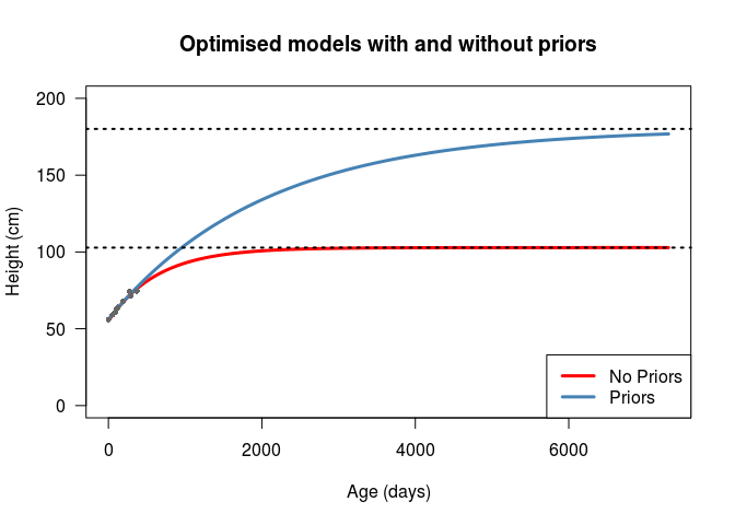
The model with no priors shows an adult (asymptotic) height of \(H_\infty = 102.83\), meaning that my son is forecast by this model to be a little bit over 1 metre tall. Looking at the graph, we can see that he’s going to reach that height at about 2000 days, or 5.5 years old, influenced by a growth rate parameter of \(K = 0.57\). Given that both my wife and I are taller than this, and we know of no reasons why we would expect him to be under the first percentile for height, I don’t fully believe this model. On the other hand, we have the model with priors predicting my son will reach his adult height of \(H_\infty = 180.12\) at about 20 years of age, with a much lower growth rate \(K = 0.18\). Although the second model is guided by subjective prior distributions, I believe it more - not only because it’s almost exactly my height, but also because aside from the value of \(K\) the model parameters are very close, and the negative-log-posterior values are also very close.
Conclusion
| j | height | weight |
|---|---|---|
| 1 | 56.0 | 3.8 |
| 3 |
|
3.5 |
| 4 |
|
3.4 |
| 15 |
|
4.0 |
| 18 |
|
4.1 |
| 25 |
|
4.1 |
| 29 |
|
4.3 |
| 39 |
|
4.9 |
| 46 |
|
5.0 |
| 50 | 59.0 |
|
| 59 |
|
5.1 |
| 74 |
|
5.3 |
| 81 | 60.5 | 5.4 |
| 86 | 60.5 | 5.6 |
| 101 | 62.5 | 5.9 |
| 122 | 64.0 | 6.0 |
| 192 | 68.0 | 7.0 |
| 276 | 74.5 | 8.3 |
| 296 | 71.5 | 8.5 |
| 373 | 74.5 | 9.6 |
So, there we go. I fit a von Bertalanffy growth model to height observations from my son’s health appointments over the first year of his life (data to the right). My aim was to (1) see how well human growth data fit the vonB mode, and (2) predict his adult height from observations now. I found that the vonB model fits human growth data very well, at least during the first year of life where a single growth regime is present (Karlberg 1987). On the other hand, I found extrapolating beyond the first year problematic, and required subjective prior distributions on leading parameters to achieve a sensible height prediction.
The high growth rate of infants is likely the reason that the model without priors estimates a high \(K\) value, reaching \(H_\infty\) sometime during childhood. According to the ICP model, infants have a high but rapidly decreasing growth rate, which is replaced by a lower, more stable, rate in childhood, and another different rate during puberty, before adult height is reached (Karlberg 1987). Later stages have a “humpy” growth pattern, where humps correspond to growth spurts during childhood and puberty.
Further work could be conducted to generate uncertainty in my prediction. I used a penalised likelihood method to estimate the parameters of the vonB model, with prior distributions penalising deviations from the observed height at 1 year old, and deviations from a growth rate that would produce an adult height that was similar to a weighted average of my wife’s and my own heights. Parameter estimates and the forecast are all maximum likelihood estimates (posterior modes), with no uncertainty reported. Confidence intervals could be estimated by using the delta-method, bootstrapping the residuals on each observation, or by running a Markov-Chain Monte-Carlo numerical integration of the posterior to generate full posterior distributions of all parameters and the model.
That’s all from me. Happy birthday to my son, thanks to my wife for growing him and being an awesome partner, and thanks to you for reading this nerdy Dad rant!
References
Francis, RIC Chris. 2016. “Growth in Age-Structured Stock Assessment Models.” Fisheries Research 180. Elsevier: 77–86.
Gliozzi, Antonio S, Caterina Guiot, Pier Paolo Delsanto, and Dan A Iordache. 2012. “A Novel Approach to the Analysis of Human Growth.” Theoretical Biology and Medical Modelling 9 (1). BioMed Central: 17.
Karlberg, Johan. 1987. “On the Modelling of Human Growth.” Statistics in Medicine 6 (2). Wiley Online Library: 185–92.
Schnute, Jon. 1981. “A Versatile Growth Model with Statistically Stable Parameters.” Canadian Journal of Fisheries and Aquatic Sciences 38 (9). NRC Research Press: 1128–40.
yes, I know it’s not technically a rate↩