Testing Rmd Support using a Schafer model

This is version 3 of my personal website. I’ve revised to a Hugo powered blogdown generated website for two reasons. First, it’s a static site generator, similar to Jekyll, serving to keep things simple and fast on the server side. Second, I’ve wanted to start blogging more, and I think the Rmarkdown integration with blogdown and Hugo will help smooth this out.

This post is a test post for using Rmarkdown to build a simple population dynamics model with process error, and generate some data with observation error. Pushing this post to github pages will require working out how TravisCI works, which I learned from David Selby’s Tea and Stats blog - a handy resource.

So, let’s get started by defining a function for the population dynamics model. I’m going to use a Schaefer surplus production model (Schaefer 1957). I like to define my Schafer models using optimal equilibrium values, known as \(B_{MSY}\) and \(U_{MSY}\) in the fisheries literature, as the leading parameters.

set.seed(123)

# Create a function to quickly call for generating biomass
prodMod <- function(  Umsy = 0.06, 
                      Bmsy = 42, 
                      procSigma = 0.1, 
                      obsSigma = 0.2,
                      nT = 100 )
{
  # Vectors to hold biomass and catch
  Bt <- numeric( length = nT )
  Ct <- numeric( length = nT )

  # Create a sequence of harvest rates
  Utmult <- c(seq(0.1,2,length = 20),seq(2,1, length = 20), rep(1,nT - 40) )
  Ut <- Utmult * Umsy

  # And draw process errors
  epst <- rnorm(nT-1, sd = procSigma)

  # Initialise at unfished
  Bt[1] <- 2 * Bmsy
  # Take first year's catch
  Ct[1] <- Ut[1] * Bt[1]

  # Now loop and fill remaining years
  for( t in 2:nT )
  {
    # Generate non-stochastic biomass
    Bt[t] <- Bt[t-1] + 2 * Umsy * Bt[t-1] * (1 - Bt[t-1] / Bmsy / 2) - Ct[t-1]
    # Add process errors
    Bt[t] <- Bt[t] * exp( epst[t-1])
    # Take catch
    Ct[t] <- Bt[t] * Ut[t]
  }

  # Draw observation errors
  deltat <- rnorm(nT, sd = obsSigma)

  # Generate absolute index of biomass
  It <- Bt * exp(deltat)

  # Return biomass, catch and model time dimension
  outList <- list(  Bt = Bt,
                    It = It,
                    Ct = Ct,
                    nT = nT )
}

# Generate the biomass
popSP <- prodMod()

# Plot the biomass and catch
plot( x = 1:popSP$nT, y = popSP$Bt, xlab = "Year", ylab = "Biomass and Catch",
      ylim = c(0,max(popSP$Bt)), type = "l", col = "red", lwd = 2, las = 1  )
  rect( xleft = 1:popSP$nT-.3, xright = 1:popSP$nT + .3,
        ybottom = 0, ytop = popSP$Ct, col = "grey40", border = NA )
  points( x = 1:popSP$nT, y = popSP$It, pch = 21, col = "grey60",
          cex = .8 )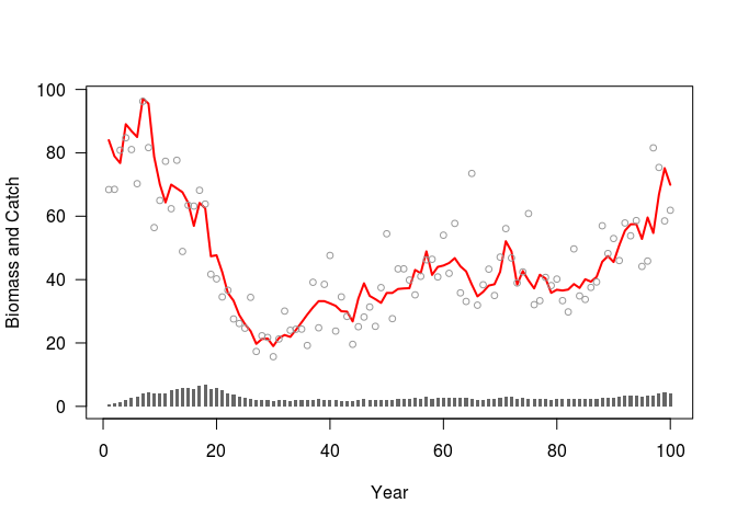

Our figure shows a 2-way trip, which describes how the biomass declines at first (the first way), then comes back up as catch is decreased (the second way). This is an ideal data set for fisheries stock assessment, as there is contrast in the catch and biomass, making it informative about both the scale of the biomass, helping to estimate \(B_{MSY}\), and the productivity of the stock, helping to estimate \(U_{MSY}\).

The next part of this post will fit a TMB model to the data generated from the above biomass. I ran this same tutorial in a seminar for our lab group at SFU this past fall, so I’ll be copying and pasting the code in from there.